https://www.pinecone.io/learn/series/image-search/zero-shot-image-classification-clip/

Both CLIP models are optimized during pretraining to align similar text and images in vector space. It does this by taking image-text pairs and pushing their output vectors nearer in vector space while separating the vectors of non-pairs.

There are three primary benefits here:

CLIP requires just image-text pairs rather than specific class labels thanks to the contrastive rather than classification focused training function. This type of data is abundant in today’s social-media-centric world. The large dataset size means CLIP can build a strong understanding of general textual concepts displayed within images. Text descriptors often describe various features of an image, not just one. Meaning a more holistic representation of images (and text) can be built.

ResNet과 비교한 CLIP의 장점

When applying a ResNet model to other domains, a standard approach is to use a “linear probe”.

여기서 linear probe란? linear probe는 사전학습된 표현은 그대로 고정해 두고, 그 위에 선형 분류기만 얹어서 학습하는 평가·전이 방식이다. 백본(예: ResNet, ViT 등)의 feature extractor는 freeze하고, 마지막 feature 벡터를 받아서 하나의 선형층(fully-connected layer, softmax 포함)을 학습한다. 새 도메인/데이터셋에 대해 이 선형층만 supervised로 학습시키므로, 백본 표현의 “선형 분리 가능성(linearly separable한지)”을 측정하는 probe 용도로 자주 쓰인다. 즉 linear probe는 새 태스크용 라벨된 샘플을 여러 개 사용하여 선형 분류기의 파라미터를 실제로 업데이트하므로 few~many-shot 학습에 해당한다.

이에 반해 CLIP은 추가로 데이터 학습이 필요하지 않으므로 zero-shot의 이점을 갖는다.

CLIP 동작 과정

• 텍스트 인코더는 주어진 텍스트를 쪼개 토큰들을 만들고 토큰끼리 셀프 어텐션을 거친다. 셀프 어텐션은 “이 패치가 어떤 다른 패치들과 같이 등장하는지, 전체 컨텍스트에서 어떤 역할인지”를 학습하게 하며, 이 global 문맥 정보는 토큰 임베딩에 삽입된다.
• 비전 인코더도 한 장의 이미지를 여러 패치 토큰들로 나눈 뒤 패치 토큰끼리 셀프 어텐션을 거친다.
• 이미지 패치 토큰과 텍스트 토큰 간의 유사도 행렬(Cross-Modal Similarity)을 구한다.

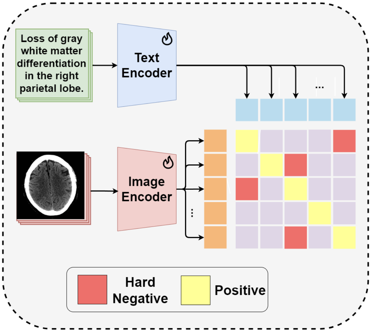
참고로 일반적인 CLIP은 이미지 한 장과 문장 전체를 하나의 벡터로 만들어 비교하지만, 사진 속 DHN-NCE은 토큰 단위로 비교하는 local-to-local alignment 방식을 쓴다.

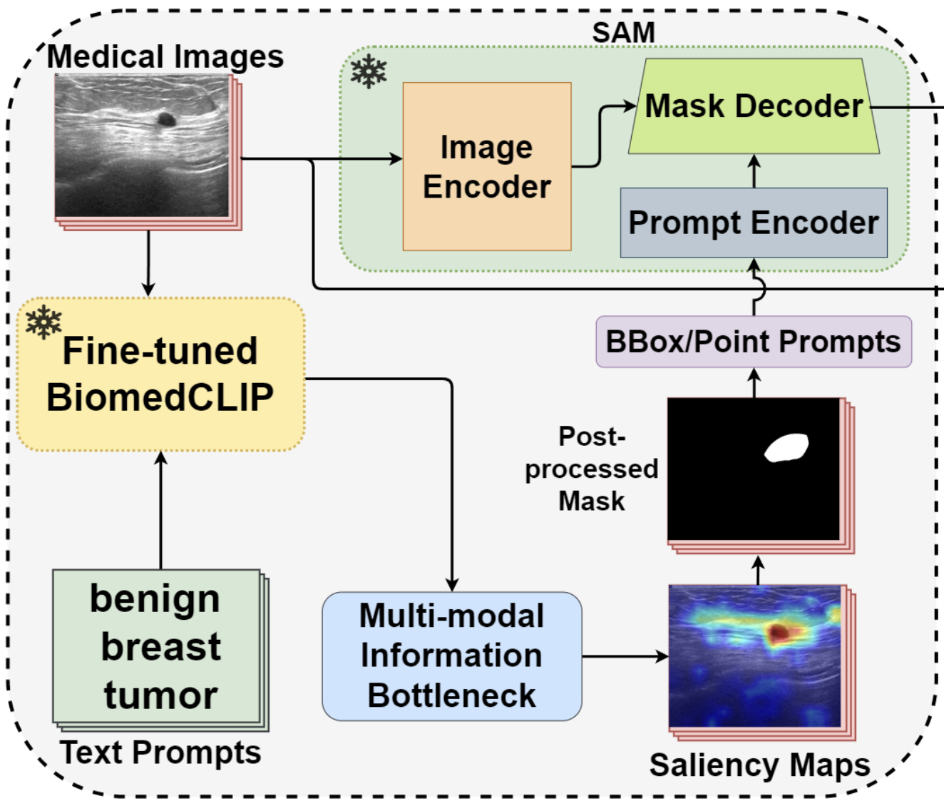
더 나아가 MedCLIP-SAM은 CLIP으로 구한 토큰 간 유사도 행렬을 M2I에 넘겨 saliency map을 생성한다.

self-attention의 활용

CLIP 모델은 텍스트와 비교하기 위해 이미지 전체를 대표하는 하나의 벡터가 필요하다. 이때 셀프어텐션 정보가 결정적으로 사용되는데

• CLS 토큰: 입력 시 추가된 CLS 토큰은 셀프어텐션 과정을 통해 모든 패치 토큰으로부터 중요한 정보를 집약한다. 최종 레이어의 CLS 토큰은 모든 패치의 어텐션 가중치가 반영된 ‘정보의 요약본’인 셈이다.
• Attention Pooling: 단순히 평균을 내는 대신, 어텐션 메커니즘을 한 번 더 사용하여 중요한 패치에 더 높은 가중치를 주어 최종 임베딩을 생성한다.

InfoNCE loss

contrastive learning에서 자주 쓰이는 손실함수로, 여기서 ‘대조’는 단순히 정답에 대한 점수를 높이기보다 정답과 오답의 점수를 ‘벌리는 데’ 초점을 둔다. 텍스트-이미지 토큰 내적의 단순합을 손실함수로 사용하지 않는 이유도 여기에 있다. 대신 대조, 즉 비교를 위해 정답과 오답의 비율을 나타내는 분수 형태를 쓴다.

또한 InfoNCE 수식의 로그-소프트맥스 구조는 칸들(두 토큰의 내적을 원소로 하는) 사이에 상호 배타적인 경쟁을 붙이게 한다. 단순히 다 더하는게 아니기 때문에 hard negative에 큰 패널티를 부여하는 효과가 있다.

\[L_{v \rightarrow t} = -\sum_{i=1}^{B} \log \frac{\exp(\mathbf{I}_{p,i}^{\top}\mathbf{T}_{p,i}/\tau)}{\sum_{j=1}^{B} \exp(\mathbf{I}_{p,i}^{\top}\mathbf{T}_{p,j}/\tau)}\] \[L_{t \rightarrow v} = -\sum_{i=1}^{B} \log \frac{\exp(\mathbf{T}_{p,i}^{\top}\mathbf{I}_{p,i}/\tau)}{\sum_{j=1}^{B} \exp(\mathbf{T}_{p,i}^{\top}\mathbf{I}_{p,j}/\tau)}\]

$L_{v \rightarrow t}$ (Image-to-Text)

• 한 이미지에 대해 어떤 텍스트들과 어울리고 그렇지 않은지 측정하는 과정

$L_{t \rightarrow v}$ (Text-to-Image)

• 한 텍스트에 대해 어떤 이미지들과 어울리고 그렇지 않은지 측정하는 과정
• 두 수식 모두 분자는 긍정쌍들의 합으로 같지만 분모는 I,T의 첨자가 다르다.

\[\text{Loss} = \frac{L_{v \rightarrow t} + L_{t \rightarrow v}}{2}\]

CLIP은 위 두 방향의 손실을 더한 뒤 평균하여 최종 손실함수로 사용한다.

DHN-NCE loss

Decoupling Positives and Negatives : 기존 InfoNCE 손실에서는 분모에 긍정 쌍과 부정 쌍이 모두 포함되어, 긍정 쌍의 유사도가 높을 경우 부정 쌍에 대한 그래디언트가 희석될 수 있다. 이를 해결하기 위해 긍정 쌍을 분모에서 제거하여 부정 쌍에 대한 학습에 더 집중하도록 한다.

Applying Hardness Weights : 의료 영상에서는 앵커 샘플(anchor sample)과 유사하지만 다른 경우(hard negatives)를 구분하는 것이 중요하며, 이러한 어려운 부정 샘플에 더 큰 페널티를 부여하는 가중치 함수를 도입한다.

• anchor sample : 대조학습에서 비교의 기준이 되는 샘플
• positive sample : 앵커 샘플과 의미론적으로 동일하거나 흡사한 샘플
• negative sample : 앵커 샘플과 의미론적으로 다른 샘플, hard negative는 그 부정 샘플 중에서도 앵커 샘플과 구별이 어려운 샘플

\[W_{v \rightarrow t}(\mathbf{I}_{p,i}, \mathbf{T}_{p,j}) = (B-1) \times \frac{\exp(\beta_1 \mathbf{I}_{p,i}^{\top} \mathbf{T}_{p,j} / \tau)}{\sum_{k \neq i} \exp(\beta_1 \mathbf{I}_{p,i}^{\top} \mathbf{T}_{p,k} / \tau)}\]

$\beta$ (Hardness Parameter): ‘어려움’의 정도를 조절하는 파라미터

분리(Decoupled)와 어려운 음성 샘플 가중치(Hard Negative Weighting)가 결합된 최종 DHN-NCE 손실함수는 다음과 같이 쓸 수 있다.

\[L_{v \rightarrow t} = -\sum_{i=1}^{B} \frac{\mathbf{I}_{p,i}^{\top}\mathbf{T}_{p,i}}{\tau} + \sum_{i=1}^{B} \log \left( \sum_{j \neq i}^{B} \exp(\mathbf{I}_{p,i}^{\top}\mathbf{T}_{p,j}/\tau) \cdot W_{v \rightarrow t}(\mathbf{I}_{p,i}, \mathbf{T}_{p,j}) \right)\] \[L_{t \rightarrow v} = -\sum_{i=1}^{B} \frac{\mathbf{T}_{p,i}^{\top}\mathbf{I}_{p,i}}{\tau} + \sum_{i=1}^{B} \log \left( \sum_{j \neq i}^{B} \exp(\mathbf{T}_{p,i}^{\top}\mathbf{I}_{p,j}/\tau) \cdot W_{t \rightarrow v}(\mathbf{T}_{p,i}, \mathbf{I}_{p,j}) \right)\]

왜 양방향 손실함수를 모두 고려할까?

수학적으로 InfoNCE 손실 함수는 이미지 $V$와 텍스트 $T$ 사이의 상호 정보량(Mutual Information)의 Lower Bound을 최대화하는 과정이라고 한다. 단방향($I \rightarrow T$) CLIP은 이미지 $i$가 주어졌을 때 정답 텍스트 $i$를 찾을 조건부 확률 $P(T|I)$만 최적화하는데, 양방향을 고려하면 $P(T|I)$와 $P(I|T)$를 동시에 최적화하게 된다.